Bayesian synthesis of probabilistic programs for automatic data modeling

Recently, I have been working on the how to combine program synthesis and probabilistic inference. Turns out that there are a variety of ways to do this:

1. You can use apply probabilistic inference for program synthesis.
2. You can apply program synthesis for probabilistic modeling.
3. And finally, you can use probabilistic inference for program synthesis to synthesize probabilistic programs.

Bayesian Synthesis of Probabilistic Programs for Automatic Data Modeling captures (3) quite nicely and in a self-contained manner. I tried reproducing (part of it) in a small notebook in this repo.

While the notebook captures the implementation details of the paper, implementations aren’t everything: there are also theoretical foundations, what are some core assumptions? What are the settings in which this works well and not? I try to capture some of these in this post.

Problem statement

We start with two things:

1. A language $\mathcal{L}$ (that we are going to formalize later with a Tagged probabilistic context-free grammar).
2. A domain $\mathcal{X}$ (the space of data that we are going to model).

The domain $\mathcal{X}$ is a set of data points $x \in \mathcal{X}$, and it also depends on which domain we are working with and is pretty straightforward to define, so we’ll focus on the tough meat: the language’s semantics.

The Language’s semantics

Let’s also say that everything in this language is an expression $E \in \mathcal{L}$. The paper would define two semantics associated with this language:

1. The prior semantic function $\texttt{Prior}: \mathcal{L} \to (0, 1]$ that calculate the prior probability of each expression.
2. The likelihood semantic function $\texttt{Lik}: \mathcal{L} \to (\mathcal{X} \to \mathbb{R}_{\geq 0})$ that calculate the likelihood of an expression given a data point. Here, $\mathbb{R}_{\geq 0}$ is the set of non-negative real numbers.

Intuitively, the prior would say how likely an expression is to be generated from the language, and the likelihood would say, given expression $E$, how likely it is to generate a data point $x \in \mathcal{X}$.

$\textbf{Bounded and Normalized}$: For the prior and likelihood to be well-defined probabilistic distributions, they must be bounded (there exists a finite upper bound) and normalized (all the probabilities sum to 1). A huge chunk of the paper is devoted to saying that:

Given a Tagged PCFG $\mathcal{G}$, the prior and likelihood functions are bounded and normalized.

Posterior semantic function: Given that both the prior $\texttt{Prior}$ and the likelihood $\texttt{Lik}$ are bounded and normalized, we can define the posterior semantic function $\texttt{Post}: \mathcal{L} \to (\mathcal{X} \to \mathbb{R}_{\geq 0})$. Recall that according to Bayes’ rule: \(\mathsf{Post}\llbracket E \rrbracket(X) = \frac{\mathsf{Prior}\llbracket E \rrbracket \cdot \mathsf{Lik}\llbracket E \rrbracket(X)}{\sum_{E' \in \mathcal{L}} \mathsf{Prior}\llbracket E' \rrbracket \cdot \mathsf{Lik}\llbracket E' \rrbracket(X)}\) For each $X \in \mathcal{X}$, define $c_X ::= \sum\limits_{E \in \mathcal{L}}\mathsf{Lik}\llbracket E \rrbracket(X) \cdot \mathsf{Prior} \llbracket E \rrbracket$ to be the marginal probability of $X$ (which is finite by assumption). Then, we can rewrite the posterior semantic function as: \(\mathsf{Post}\llbracket E \rrbracket(X) = \frac{\mathsf{Prior}\llbracket E \rrbracket \cdot \mathsf{Lik}\llbracket E \rrbracket(X)}{c_X}\)

Now we are finally ready to state the problem:

Objective 3.5 (Bayesian Synthesis) Let $\mathcal{L}$ be a language whose denotational semantics $\mathsf{Prior}$ and $\mathsf{Lik}$ satisfy 3.1., 3.2., and 3.3. Given a dataset $X \in \mathcal{X}$, generate expressions $E$ with probability $\mathsf{Post}\llbracket E \rrbracket(X)$.

Bayesian relies on posterior distributions to infer new $E$, but here’s a problem: even though $\mathsf{Post}\llbracket E \rrbracket(X)$ is bounded and normalized, it is not tractable to compute for all $E \in \mathcal{L}$ and $X \in \mathcal{X}$.

Markov Chain Monte Carlo to the rescue

Bayesian inference doesn’t work if we can’t calculate the posterior distribution. But we do know how well each expression $E$ does at modeling the data point $X \in \mathcal{X}$. This is exactly the settings which Markov Chain Monte Carlo (MCMC) handles, specifically, the Metropolis-Hastings algorithm. Only requires you to say how “relatively well” each sample is compared to the previous one, along with a proposal distribution that generate new sample from the previous one. For our case, we already know the likelihood $\mathsf{Lik}\llbracket E \rrbracket(X)$, we just need a proposal distribution $\mathcal{T}$ that generates new expressions $E’$ from the previous one $E$, conditioned on the language’s likelihood $\mathsf{Lik}\llbracket E \rrbracket(X)$ and the language’s prior $\mathsf{Prior}\llbracket E \rrbracket$.

Let’s break this down:

1. $\text{SelectRandomElementUniformly}(A_E)$ is a function that randomly selects a node in the parse tree $E$. When you have an expression $E$ defined in accordance with a PCFG, you can always pick a random terminal in the AST (the parse tree of the expression $E$).
2. $\text{Sever}_a\llbracket E \rrbracket$ is a function that severs the parse tree $E$ at the node $a \in A_E$. Basically, one example of this is if you have an expression $E = (\cdot\ x\ y)$, and you select the node $a = (1)$ - meaning the 1st child of the root node, then $\text{Sever}_a\llbracket E \rrbracket = (Variable, (\cdot\ \square\ y)$. Where $Variable$ is a non-terminal symbol in the PCFG that are used to produce terms like $x, y, z$, etc.
3. $\text{Expand}\llbracket \cdot \rrbracket(N_i)$ is a function that expands the non-terminal symbol $N_i$ in the parse tree $E$ in accordance with the PCFG’s probability distribution. We will be defining this below.
4. Let’s call $\alpha(E, E’)$ the probability of accepting the mutation, defined as \(\alpha(E, E') = \min\left\{1,\left(\lvert A_E\rvert/\lvert A_{E'}\rvert\right)\cdot(L'/L)\right\}\).

$\color{lightgreen}Question$: Why it’s called algorithm 2? Why not algorithm 1?

$\color{lightgreen}Answer$: Algorithm 1 is the main algorithm that uses algorithm 2!

Markov Chain in general relies on drawing many samples from the chain to approximate the stationary distribution. The more samples we draw, the more accurate the approximation. So algorithm 1:

Metropolis-Hastings relies on the property that, if the chain is irreducible (does not have any absorbing states) and aperiodic (does not have any cycles), then it will converge to a unique stationary distribution. By defining the transition based on the PCFG’s proability distribution, we can guarantee that the chain is irreducible and aperiodic.

Defining $\text{Expand}\llbracket \cdot \rrbracket(N_i)$ and $\mathcal{T}$

We will now define formally the prior $\mathsf{Prior}$ and then $\mathsf{Expand}\llbracket \cdot \rrbracket(N_i)$ accordingly. For that, we need to define a tagged probabilistic context-free grammar (PCFG) $G$, in the paper:

$\color{lightgreen}\textbf{Definition 4.1. (Tagged PCFG with Random Symbols)}$. Let $G = \langle \Sigma, N, R, T, P, Q, S\rangle$ denote a tagged PCFG with terminals, non-terminals, and production rules.

• $\color{lightgreen}R ::= \{R_{ik} \mid i=1, \ldots, m; k=1, \ldots, r_i\}$ is a set of production rules, where $R_{ik}$ is the $k^\text{th}$ production rule of non-terminal $N_i$. Each production rule $R_{ik}$ is a tuple of the form:

\[R_{ik} ::= \langle N_i, T_{ik}, \tilde{N}_1, \ldots, \tilde{N}_{h_{ik}} \rangle \qquad \color{yellow}(6)\]

Where $h_{ik} \geq 0$ is the numer of non-terminal on the rhs. If the set of $\tilde{N}$ is not empty, this is called recursive production rule.

• $\color{lightgreen}T$ is a set of phrase tag symbols, disjoint from $N$, where $T_{ik}$ is a unique symbol identifying the production rule $R_{ik}$
• $\color{lightgreen}P: T \to (0, 1]$: phrase tag symbols to their probabilities.
• $\color{lightgreen}Q: T \times \Sigma \to [0, 1]$ map from phrase tags and terminal symbols to probabilities, where $Q(T_{ik}, s)$ is the probaiblity that production rule $R_{ik}$ of non-terminal $N_i$ draws the terminal symbol $s \in \Sigma$. For each tag $T_{ik}$, the probabilities over symbols sum to unity $\sum\limits_{s \in \Sigma}Q(T_{ik}, s) = 1$.
• $\color{lightgreen}S \in N$ is a designated start symbol.

We additionally assume that grammar $G$ is proper: production rules must be cycle-free, and there are no useless symbols in $\Sigma \cup N \cup T$.

Basically, we would have a probability assigned to each production rule $R_{ik}$ ($Q(T_{ik}, s)$) that say, “here is the probability that we would expand in this direction”, and also a prior to say which non-terminal symbol $N_i$ we would expand to ($P(T_{ik})$).

$\color{lightgreen}\textbf{Expand:}$ Finally, $\mathsf{Expand}: \mathcal{L}(G) \to N \to [0, 1]$ is defined inductively: \(\begin{array}{c} \mathsf{Expand}\llbracket (T_{ik}\ s) \rrbracket (N_i) := P(T_{ik}) Q(T_{ik}, s)\\ \mathsf{Expand}\llbracket (T_{ik}\ E_1 \cdots E_{h_{ik}}) \rrbracket (N_i) := P(T_{ik}) \cdot \prod_{z=1}^{h_{ik}} \mathsf{Expand} \llbracket E_z \rrbracket (\tilde N _z) \end{array}\) Where $R_{ik} = (T_{ik}, N_i, \tilde{N}_1, \ldots, \tilde{N}_{h_{ik}})$, for $i= 1,\ldots, n$ and $k= 1, \ldots, r_i$.

$\color{lightgreen}\textbf{Proposal Distribution/Transformation Operation }\mathcal{T}:$ How do we define the operation that gives us (1) a new expression $E’$ from the current expression $E$ (so that it creates a chain) and (2) gives us the probability how likely we can obtain $E’$ from $E$?

The authors (Feras A. Saad et al.) deals with this by severing this “transformation” (or as software engineer people often use the term “mutation” since the original infamous GenProg paper) into two steps: severing and expansion.

Intuitively, severing means that, taken an expression $E$, you cut out part of the expression. Specifically, this is done by first creating a set of all indices for each expression $E$. In the original paper:

Define the set $A ::= {(a_1, a_2, \ldots, a_l) \mid a_i \in {1, 2, \ldots, h_{\max}}, l \in {0, 1, 2, \ldots, }}$ to be a countably infinite set that index the nodes in the parse tree of $E$, where $h_{\max}$ denotes the maximum number of symbols that appear on the right of any given production rule of the in $(6)$.

Each element $a \in A$ is a sequence of sub-expression positions on the path from the root node of a parse tree to another node. For example, if $E = (t_0\ E_1\ E_2)$ where $E_1 = (t_1\ E_3\ E_4)$ and $E_2 = (t_2\ E_5\ E_6)$, then the root node of the parse tree has index $a_\text{root} ::= ()$; the node corresponding to $E_1$ has index $(1)$, the node corresponding to $E_2$ has index $(2)$; $E_3$ and $E_4$ are $(1, 1)$ and $(1, 2)$, respectively;

and the nodes corresponding to $E_5$, $E_6$ have $(2, 1)$ and $(2,2)$. For an expression $E$, let $A_E \subset A$ denote the finite subset of nodes that exists within the parse tree of $E$.

The description of $\mathsf{Sever}$ is very interesting, and I’d recommend checking it out later. But for now, check the intuitive image below:

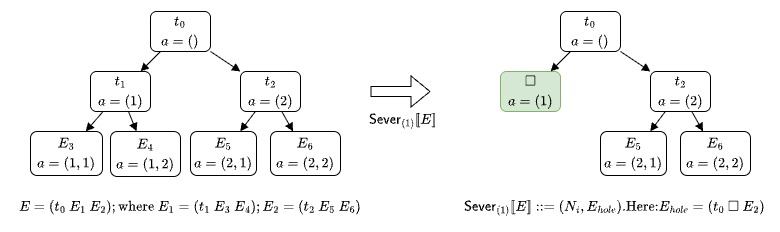
Here, we would sever the first child of the root node, resulting in the $E_{\text{hole}} = (t_0\ \square\ E_2)$, $N_i$ would be the non-terminal symbol that produced $E_1$.

In conjunction with $\mathsf{Sever}$, let us define $\mathsf{SubExpr}_a$ which is the sub-expression at the index $a$. $\mathsf{SubExpr}_a$ has to be well-defined, so for an index $a$ that is out of range, it should return the empty expression $\emptyset$, otherwise, is is inductively defined as follows: \(\mathsf{SubExpr}_a\llbracket(t\ E_1\ E_2\ \ldots\ E_l)\rrbracket ::= \left\{\begin{array}{ll} \emptyset& \text{if \(a = ()\) or \(a_1 > k\)}\\ E_j & \text{if \(a = (j)\) for some $1 \leq j \leq k$} \\ \mathsf{SubExpr}_{(a_2, a_3, \ldots )} \llbracket E_j\rrbracket & \text{if $i\neq (j)$ and $a_1 = j$ for some $1 \leq j \leq k$} \end{array}\right.\)

What’s followed by severing? Finding a new $E_{sub}’$ to fill the hole. This is where the expansion comes in. From the severing process, we would have the non-terminal symbol $N_i$ that produced $E_1$. We would then expand $N_i$ in accordance with $\mathsf{Expand}\llbracket \cdot \rrbracket(N_i)$.

Consider the probability that $\mathcal{T}$ takes an expression $E$ to another expression $E’$, which by total probability is an average over the uniformly chosen node index $a$: \(\mathcal{T}(X, E\to E') = \frac{1}{|A_E|} \sum\limits_{a \in A_E} \mathcal{T}(X, E \to E'; a) = \frac{1}{|A_E|} \sum\limits_{a \in A_E \cap A_{E'}} \mathcal{T}(X, E \to E'; a)\) where \(\mathcal{T}(X, E \to E', a) ::= \left\{ \begin{array}{l} \mathsf{Expand}\ \llbracket\mathsf{SubExpr}_a\llbracket E'\rrbracket\rrbracket(N_i) \cdot \alpha(E, E') + \mathbb{I}[E = E'](1 - \alpha(E, E'))\\ \qquad\ \text{ if \(\mathsf{Sever}_a\llbracket E\rrbracket = \mathsf{Sever}_a \llbracket E'\rrbracket = (N_i, E_\text{hole}) \) for some $i$ and $E_\text{hole}$}\\ 0\qquad\text{otherwise} \end{array} \right.\) Note that we discard terms in the sum with $a \in A_E \setminus A_{E’}$ because for these terms $\mathsf{Sever}_a\llbracket E’\rrbracket =\emptyset$ and $\mathcal{T} (X, E\to E’; a) = 0$.

This is the end. After this, the process is pretty straightforward: we would sample a new expression $E’$ from the current expression $E$ using the Metropolis-Hastings algorithm, and then we would accept or reject the new expression based on the probability of accepting the mutation (Algorithm 2). The process is repeated for $n$ times, and we would return the last expression $E_n$.

Conclusion

I tried covering the paper from a top-down perspective and I also omitted lots of details. I remember that there are moment I read the paper and just gasped at the math and how cool it is. If you find this to be interesting, I’d recommend checking out the paper for more details.