Grammars that generalize: trying to find domain-invariant bird recognition
Here’s a question Duy and I were kicking around: what if you combined a small DSL with a neural network classifier and the classifier head itself happened to be domain-invariant by construction? Not as a replacement for adaptation methods like CDAN – but as a much stronger starting point for them.
Turns out it works. We replaced a linear classification layer with a probabilistic context-free grammar over spatial layout programs. The grammar scores spatial relations between detected parts – and those relations don’t change when you go from photos to paintings.
Code: datvo06/NeuroSymbolicDG. Checkpoints: HuggingFace.
The setup and the result
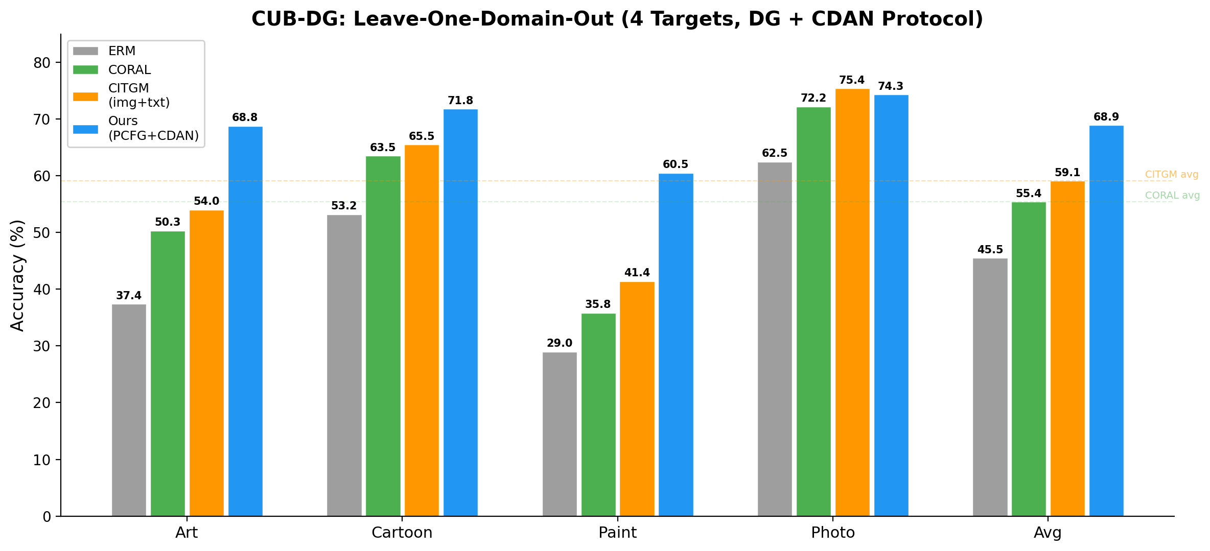
The benchmark is CUB-DG (Min et al., ECCV 2022): 200 bird species across 4 visual domains (Photo, Art, Cartoon, Paint). Train on 3 domains, test on the held-out one. Best published image-only method, CORAL (Sun & Saenko, 2016): 49.9% avg. Best with image+text, CITGM: 53.6%. We get 67.0% with image only.
The pipeline:
ResNet-50
  → 1×1 conv → k=8 heatmaps
  → spatial_soft_argmax → 8 primitives {(cx, cy, bbox, conf)}
  → PCFG: 344 productions, sparsemax weights per class
  → class scores → log-softmax
The concept bottleneck (1x1 conv + spatial soft-argmax) forces the network to decompose its representation into $k=8$ spatially localized primitives. Each primitive has a location, bounding box, and confidence. No hand-designed primitive vocabulary; the primitives emerge from end-to-end training.
Same backbone, same data, same everything – swap the PCFG head for a linear classifier:
| Method | Art | Cartoon | Paint | Avg |
|---|---|---|---|---|
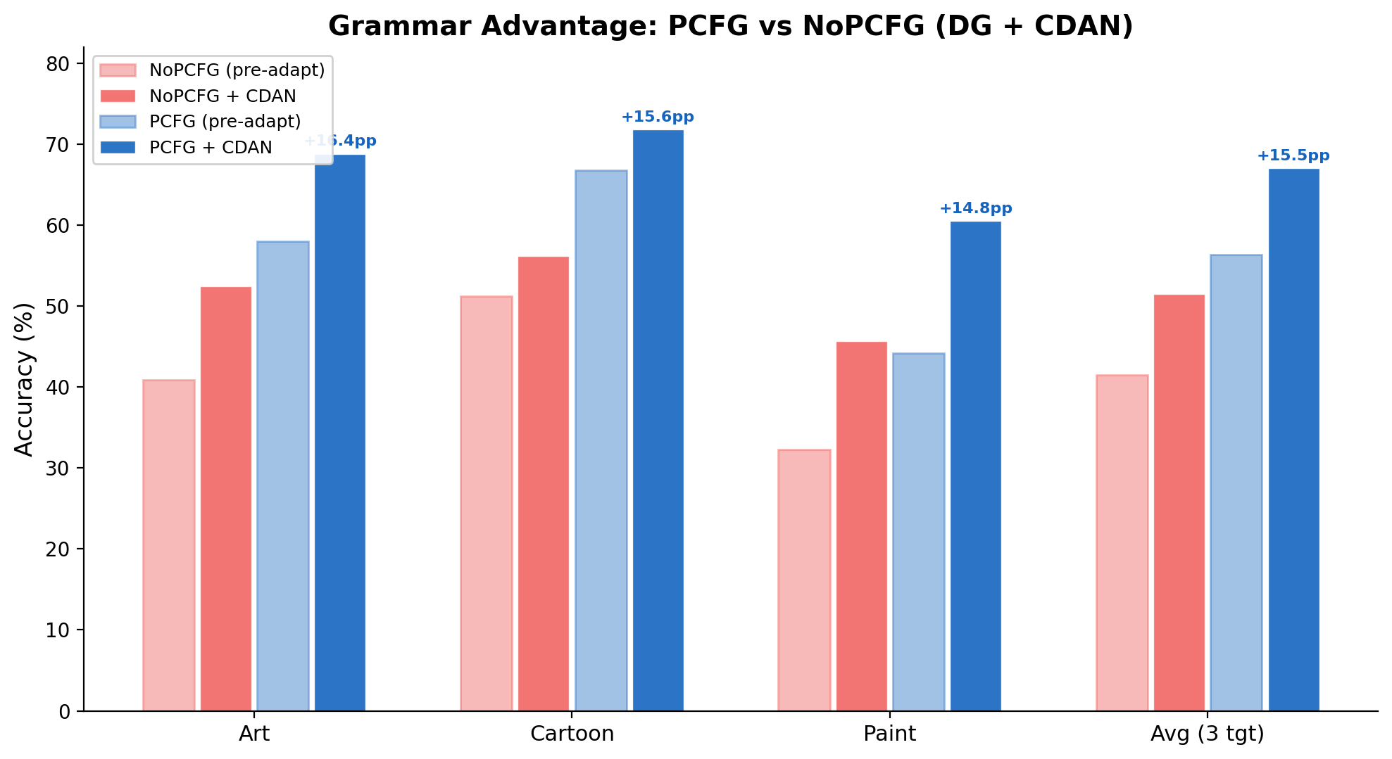
| NoPCFG+CDAN | 52.4% | 56.2% | 45.7% | 51.4% |
| PCFG+CDAN | 68.8% | 71.8% | 60.5% | 67.0% |
| Grammar $\Delta$ | +16.4 | +15.6 | +14.8 | +15.6 |
+15.6pp from changing the classifier head. The gap is remarkably consistent across targets. Now let me explain what that classifier head actually is.
The grammar
A standard classifier ends with a linear layer: backbone features $\to$ class logits. We replace that with a PCFG over a small layout DSL. The DSL has two sorts of terminals:
- Existence: $\texttt{has}(j)$ – “primitive $j$ is present” (returns its confidence $\in [0,1]$)
- Relation: $\texttt{rel}(r, i, j)$ – “primitive $i$ is in spatial relation $r$ to primitive $j$” (returns a soft score)
The spatial relations are scored by sigmoid/Gaussian kernels over detected primitive coordinates:
\[\begin{aligned} \texttt{above}(i, j) &= \sigma\bigl(\lambda_1 (cy_j - cy_i - m_1)\bigr) \\ \texttt{left\_of}(i, j) &= \sigma\bigl(\lambda_2 (cx_j - cx_i - m_2)\bigr) \\ \texttt{near}(i, j) &= \exp\bigl(-\|c_i - c_j\|^2 / 2\rho^2\bigr) \\ \texttt{aligned\_h}(i, j) &= \exp\bigl(-(cy_i - cy_j)^2 / 2\tau_1^2\bigr) \\ \texttt{aligned\_v}(i, j) &= \exp\bigl(-(cx_i - cx_j)^2 / 2\tau_2^2\bigr) \\ \texttt{contains}(i, j) &= \sigma\bigl(\lambda_3 \min(\text{margin}_{ij})\bigr) \end{aligned}\]All parameters $(\lambda, m, \tau, \rho)$ are learnable – jointly optimized with the rest of the network. The geometry of “above” and “near” adapts to the data; we don’t hand-code thresholds.
Given $k=8$ primitive types and 6 relation types, the universal grammar enumerates all possible spatial constraints:
\[\begin{aligned} \texttt{Constraint} &\to \texttt{has}(p_j) && \text{for } j \in \{0, \ldots, 7\} && \text{(8 productions)} \\ \texttt{Constraint} &\to \texttt{rel}(r, p_i, p_j) && \text{for } r \in \mathcal{R},\; i \neq j && \text{(6 × 56 = 336 productions)} \\ \texttt{Layout}_y &\to \texttt{choice}(\texttt{score}(w_1, c_1), \ldots, \texttt{score}(w_{344}, c_{344})) && && \text{(marginalization)} \end{aligned}\]344 productions total. Each class $y$ has its own weight vector $\mathbf{w}_y \in \mathbb{R}^{344}$, normalized by sparsemax (Martins & Astudillo, 2016). Unlike softmax, sparsemax produces exact zeros – each class commits to a small set of active productions (typically 4–17 out of 344, mean 8). The class score:
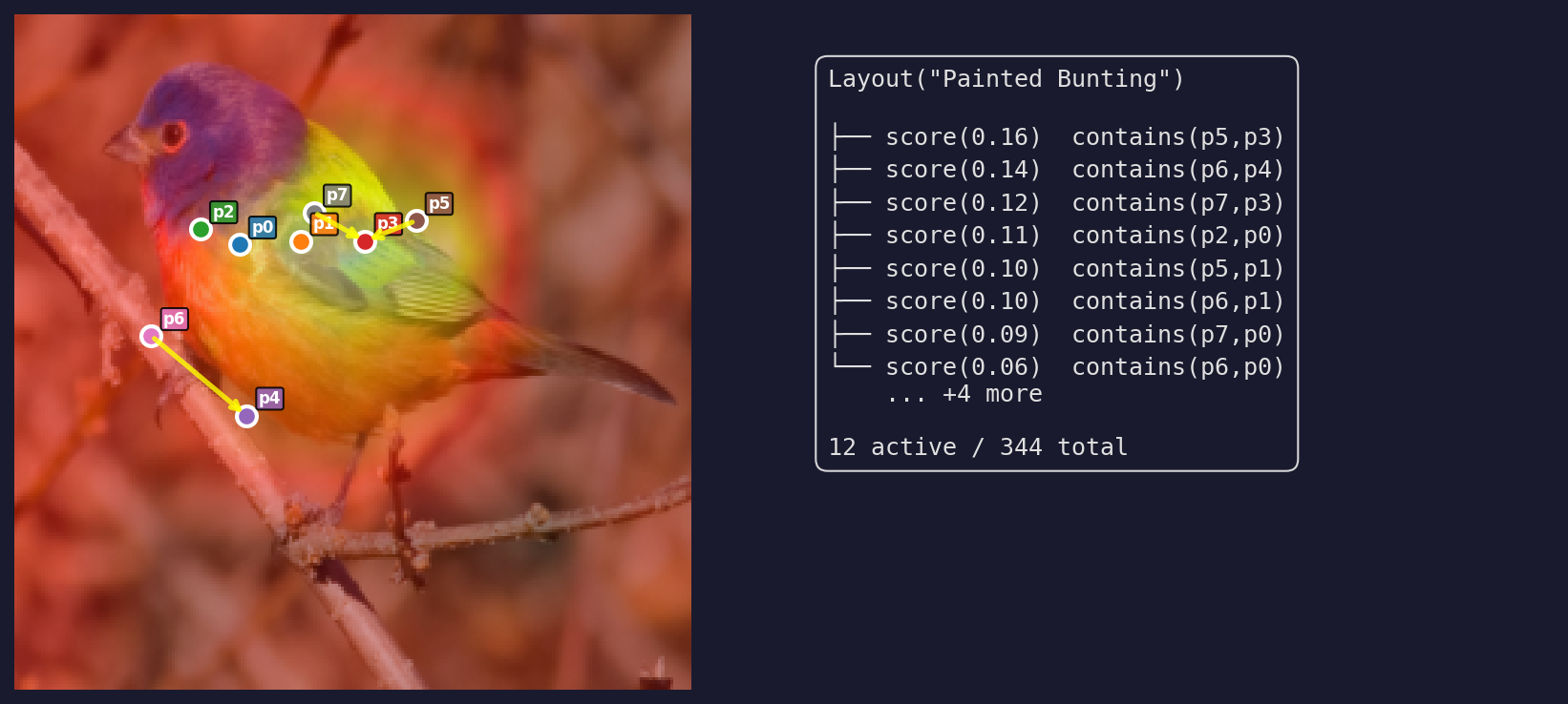
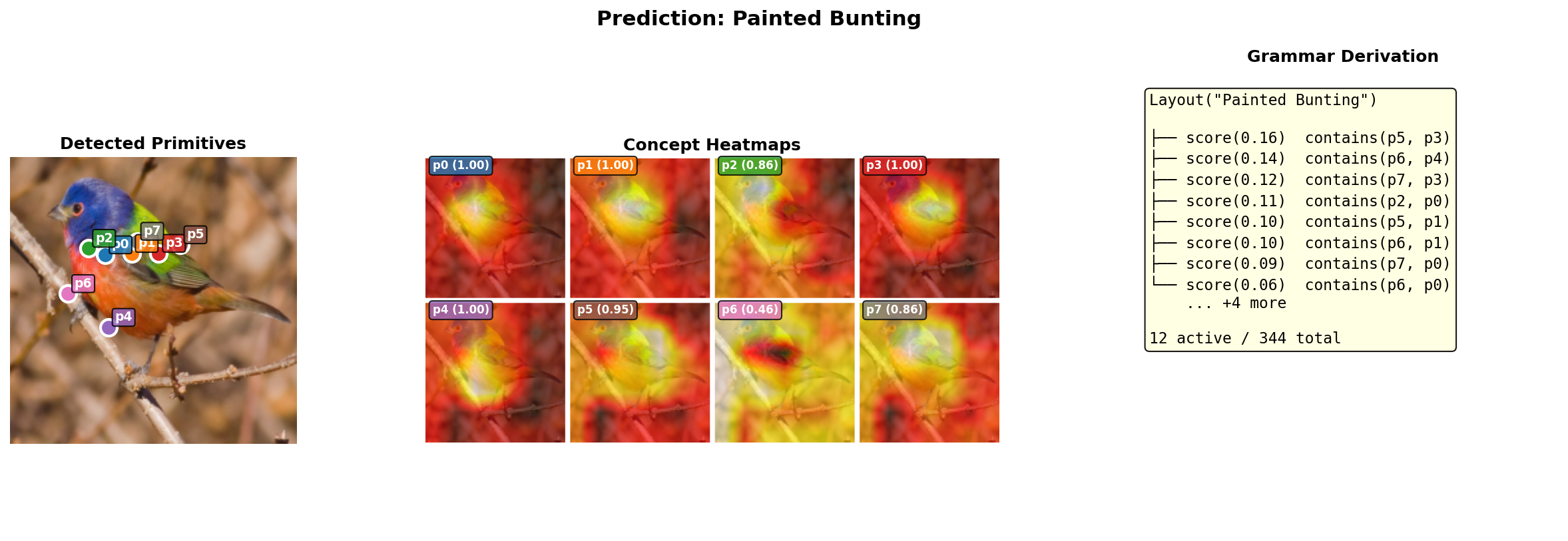
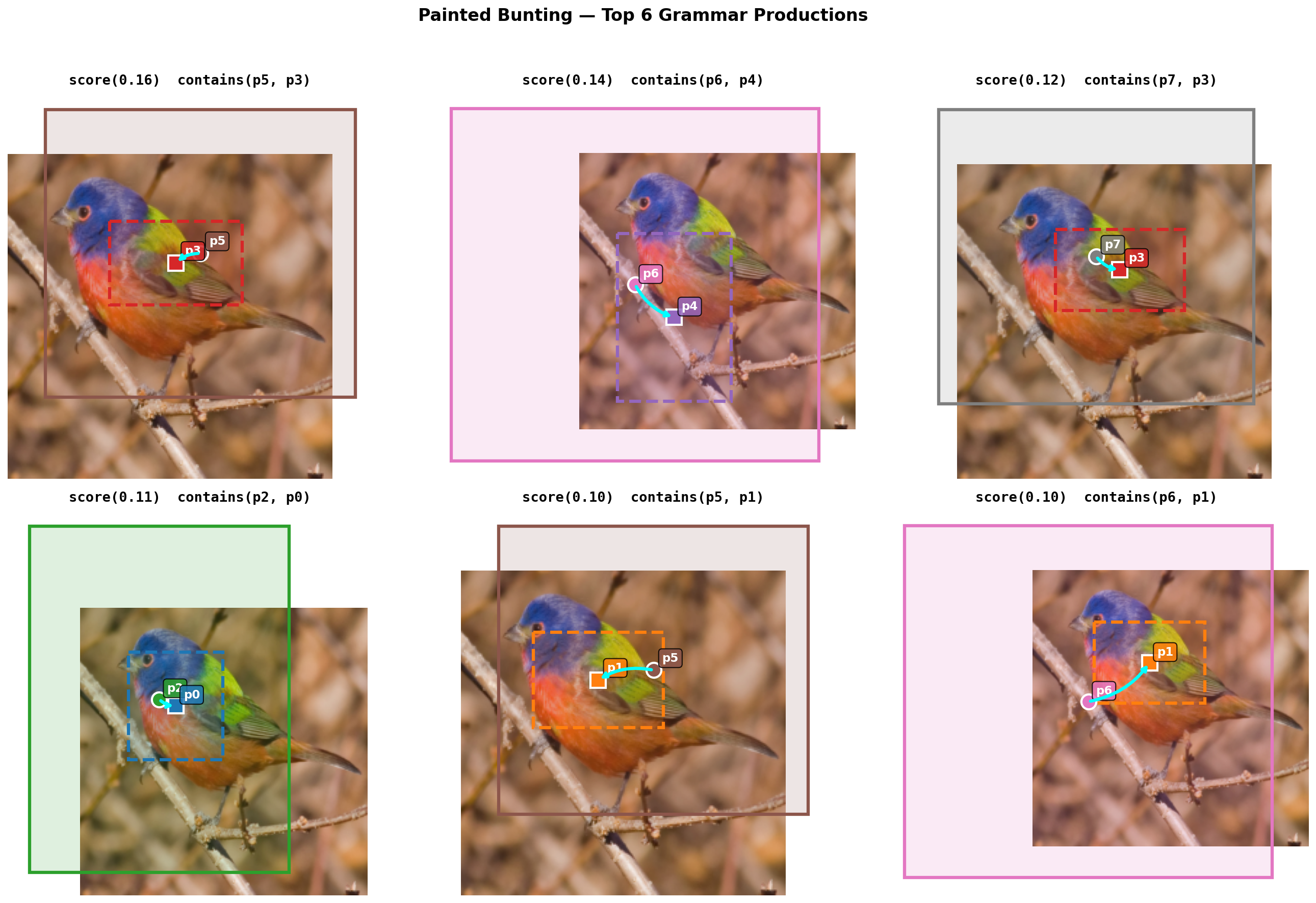
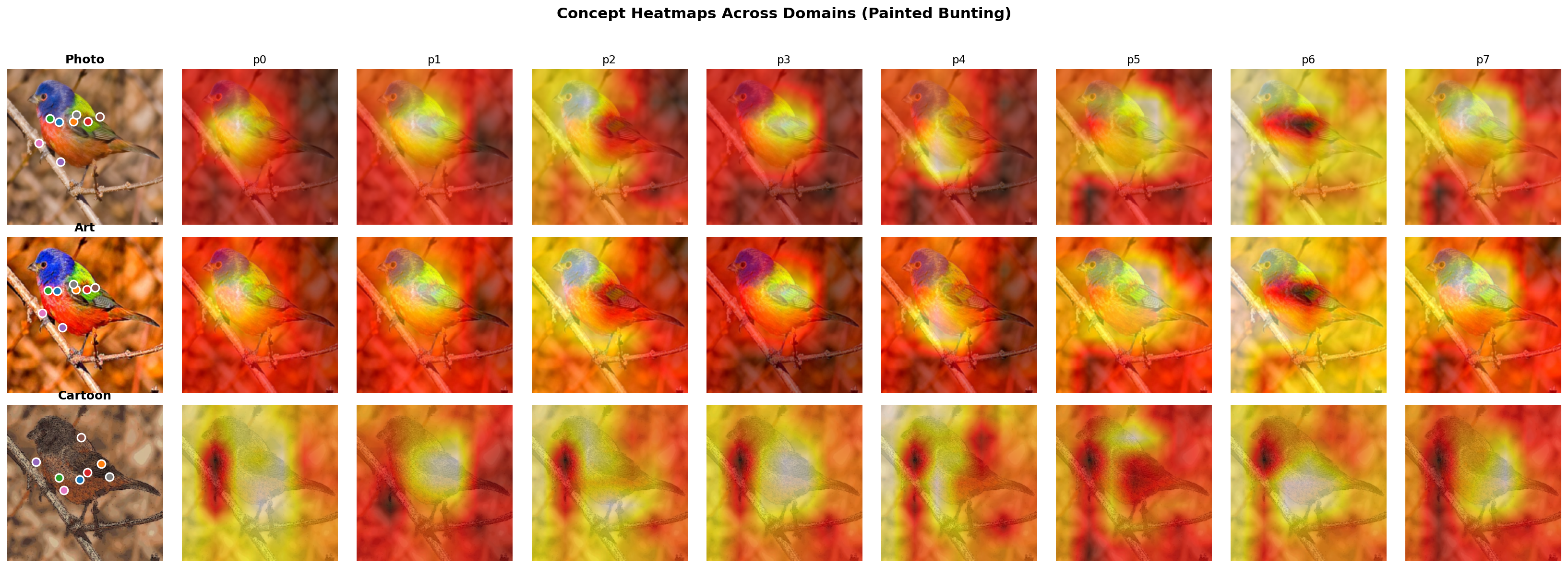
\[W_y(x) = \sum_{p=1}^{344} \underbrace{[\text{sparsemax}(\mathbf{w}_y)]_p}_{\text{grammar weight}} \cdot \underbrace{\beta_p(x)}_{\text{spatial score}}\]If you squint, this is a linear classifier over spatial relation features with sparsemax forcing each class to pick a small structural explanation. Here’s what that looks like on a real image – a Painted Bunting, from detected primitives through heatmaps to the grammar derivation:
And the top 6 grammar rules visualized spatially with bounding boxes:
Every class learns a distinct grammar. Here are 5 maximally diverse species – picked by greedy selection to minimize mutual cosine similarity:
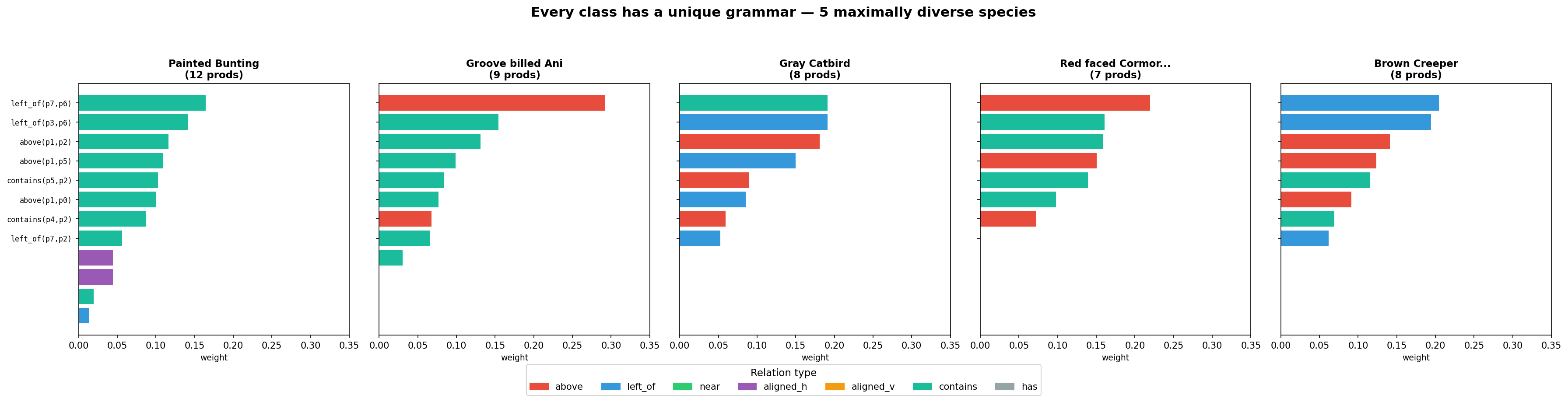
All 200 classes have unique active production sets (0 identical pairs), with a mean pairwise cosine similarity of just 0.04:
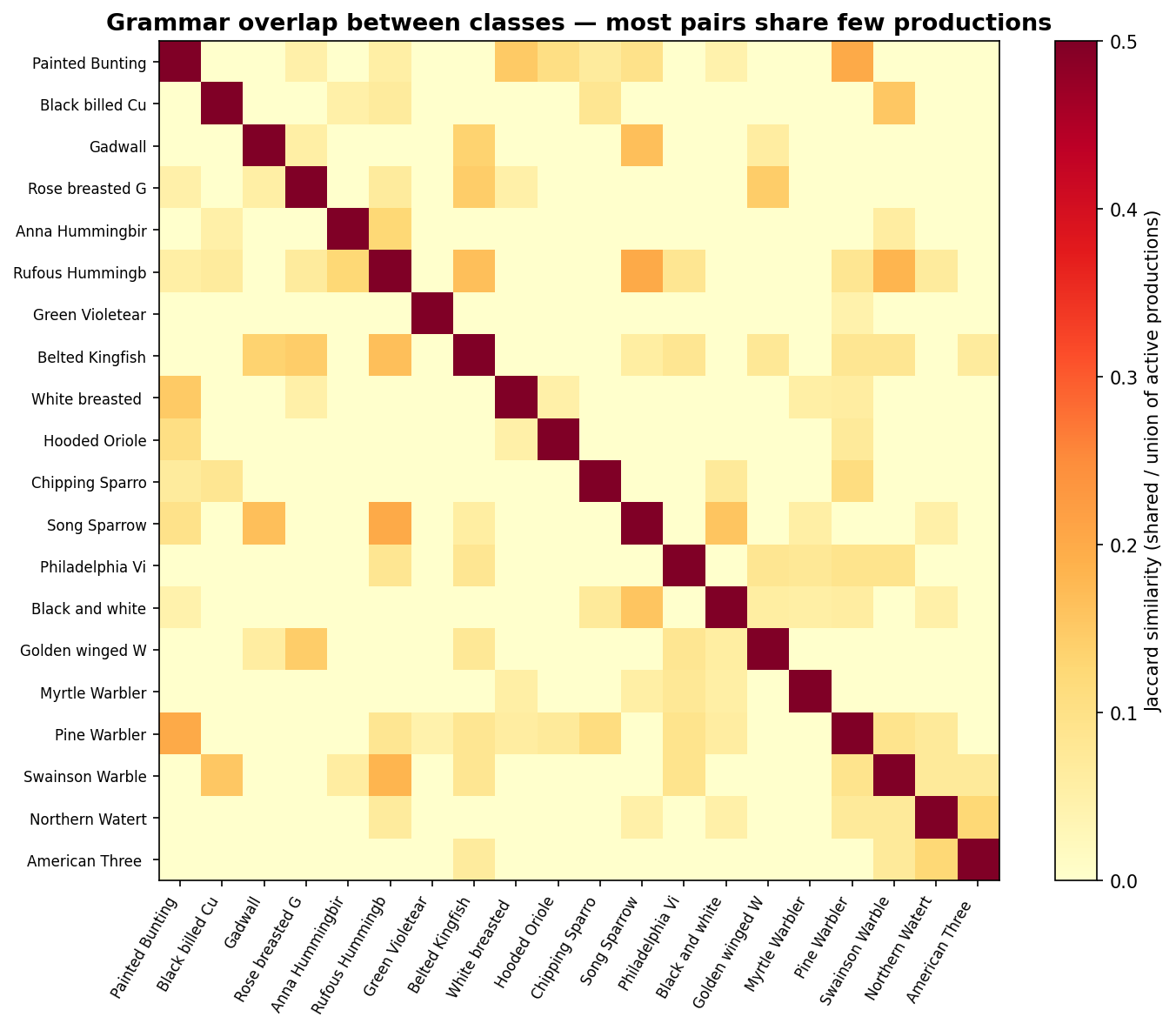
The grammar learns genuinely distinct structural descriptions per species, not a one-size-fits-all template. And since the weights are per-class not per-domain, the structural recipe for each species is identical across Photo, Art, Cartoon, and Paint – domain invariance by construction.
Why it works
If you think about it in PL terms, the grammar weights define a finite abstraction of the image. You go from a continuous pixel space to a sparse vector of spatial relation scores – a very coarse summary. Domain shift is a transformation in the concrete (pixel) domain. But the grammar’s abstraction is coarse enough to be invariant to it: “beak above breast” holds in photos and in oil paintings, even though the pixels are completely different.
Here’s the same species across Photo, Art, and Cartoon – the heatmap patterns are consistent despite dramatic appearance changes:
The grammar also discovers on its own which relations are domain-invariant:
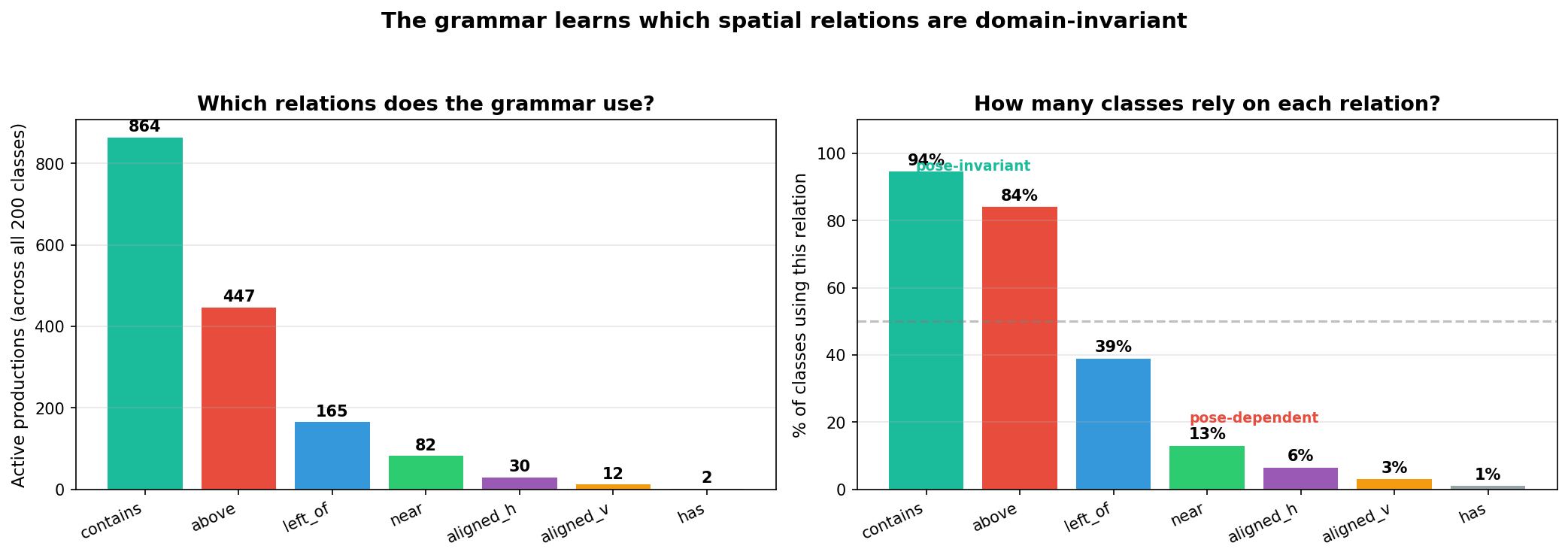
contains dominates (94% of classes), above is second (84%), left_of drops to 39%. Why? contains (really soft overlap – the bounding boxes are too diffuse for true containment) is pose-invariant: two overlapping primitives stay overlapping regardless of orientation. above holds reliably across poses. But left_of is pose-dependent – a bird facing left has its beak left-of-body; facing right, it’s reversed. The training data includes random horizontal flips, so the grammar learns to avoid it. Nobody told it left_of is unreliable – sparsemax drove it to zero.
This is also why you can’t improve it by adding alignment losses. The abstraction is already domain-invariant. Forcing additional constraints just fights with the grammar’s natural behavior.
Connection to neuro-symbolic scene understanding
This grammar is semantically similar to the visual reasoning programs in Neural-Symbolic VQA (Yi et al., 2018) and the CLEVR ecosystem (Johnson et al., 2017). Our rel("above", p3, p1) is not far from relate(above, obj3, obj1) in a CLEVR-style program. But there’s a key difference:
- CLEVR-style: the semantics are learned – a neural module learns what “left_of” means. Flexible but can overfit to the training distribution.
- Ours: the semantics are given differentiably –
above(i, j) = σ(λ(cy_j - cy_i - m))is a fixed functional form with learnable parameters. The shape of the relation is locked in (“above” really means “higher”), but the threshold adapts. This is what makes it domain-invariant by construction.
The tradeoff is expressiveness vs. invariance. For spatial relations between detected bird parts, the sigmoid/Gaussian forms are expressive enough – and the invariance is worth it.
One program, three semantics
The design principle is something that’ll look familiar if you’ve done any work with abstract interpretation: define the grammar once as an effectful program, then choose your semantics at the call site.
The grammar is implemented using effectful algebraic effects. The five DSL operations – has, rel, conj, choice, score – are declared as algebraic effects via @Operation.define. The same program runs under different handlers:
with handler(eval_handler):     score = grammar(class_idx)  # → Tensor
with handler(inside_handler):   table = grammar(class_idx)  # → InsideTable
with handler(symbolic_handler): tree  = grammar(class_idx)  # → DerivNode
The eval handler interprets the DSL in the non-negative real semiring $(\mathbb{R}_{\geq 0}, +, \times, 0, 1)$ – choice is addition, conj is multiplication, score scales by the grammar weight. Fast scalar class score.
The inside handler interprets the same program in the powerset semiring – tracking which subsets of primitives each subprogram explains. This is the inside algorithm adapted from strings to sets: $I(A, S) = \sum_{A \to B\;C} w \sum_{S = S_1 \uplus S_2} I(B, S_1) \cdot I(C, S_2)$. Exact marginals over all derivations.
The symbolic handler builds an explicit DerivNode tree – that’s how we extract the derivation visualizations above.
Same program, three abstract domains. This is the same pattern from my earlier post on Bayesian synthesis – there we had MCMC over program structures with a PCFG prior. Here, the programs are spatial layout grammars and the data is images, but the birth/death/swap moves over derivation trees are the same idea.
(In practice, we bypass effectful for training via forward_vectorized() – pure tensor ops, ~26x faster. But the handler-based version is what makes the system compositional.)
What doesn’t work, and what that tells us
We tried several things to improve on top of the grammar. They all made it worse:
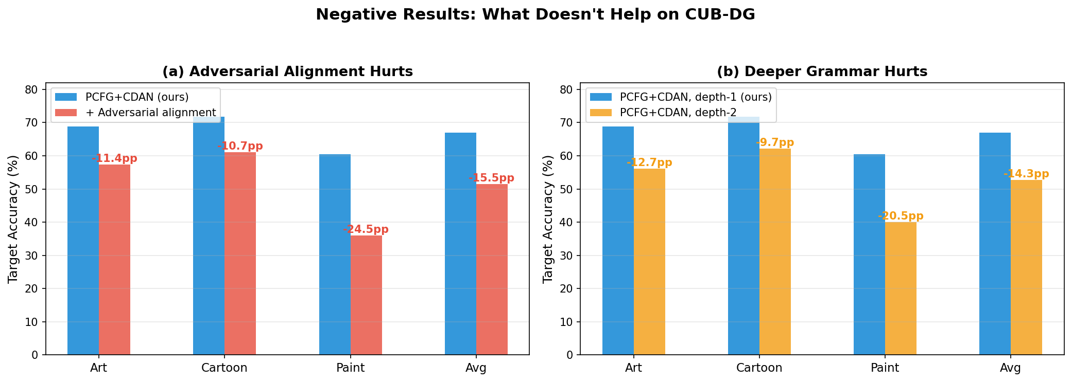
- Adversarial alignment (-5.5pp): 3-way domain discriminator (Ganin et al., 2016). The grammar already captures the right invariances; forcing alignment disrupts this.
- Deeper grammar (-4.2pp): Hierarchical sublayouts (depth-2). Overfits to source domain structure.
- Production score alignment (-12.9pp): MMD (Gretton et al., 2012) between production activations across domains. Redundant with the grammar’s compositional structure.
Now let me be honest about what this all means.
“It’s just a kernel machine with hand-designed spatial features and sparsemax. Why call it a grammar?” Partly fair. At depth-1, the PCFG is a flat weighted sum over 344 fixed productions – no recursion, no hierarchical derivation. You could rewrite the whole thing as class_score = sparsemax(W) @ spatial_features(x) and it would be mathematically identical. So why the grammar framing?
Two reasons. First, the infrastructure does more than the depth-1 config uses. The DSL, the handlers, the inside algorithm – these support genuine compositionality. We tried it (depth-2) and it hurt on this benchmark, but the machinery is there for tasks where hierarchical structure matters. Second, the grammar framing is what led us to this design. “Enumerate all pairwise spatial relations and let the model pick a sparse subset per class” is a natural consequence of thinking in terms of productions. If we’d started from “let’s design spatial kernel features,” we might have ended up somewhere similar, but we probably wouldn’t have built the handler-based architecture that makes the system extensible.
That said: if you want to call it a spatial relation feature selector with sparsemax sparsity, I won’t fight you. The results don’t change.
“The depth-2 result is the most interesting finding.” I agree. Why doesn’t compositionality help? The depth-1 abstraction is already coarse enough to be domain-invariant. Adding hierarchical structure introduces more parameters that overfit to source domain structure – the specific way parts group in photos doesn’t transfer to how they group in cartoons. The flat version avoids this by not committing to any grouping. There’s a sweet spot of abstraction granularity: coarse enough to transfer, fine enough to discriminate. Pairwise relations hit it for birds. Whether that generalizes is an open question.
“The ablation confounds architecture and features.” The PCFG head operates on 344-dim spatial features with sparsemax; the linear head operates on 2048-dim backbone features with softmax. Different capacity, different regularization, different feature space. The honest claim is: this combination of inductive biases helps, not that the grammar alone accounts for all +15.6pp. A fairer ablation would be a linear head over the same 344 spatial features, or sparsemax without the grammar structure. We didn’t run those. If someone does and the gap shrinks to 5pp, the interesting part is still which 5pp the grammar contributes and why.
“How does this compare to concept bottleneck models?” CBMs (Koh et al., 2020) also decompose representations into interpretable concepts. The difference is what sits on top. A CBM feeds concept activations into a linear classifier. We feed spatially localized primitives into a grammar that scores pairwise spatial relations. The CBM asks “which concepts are present?”; the grammar asks “how are the concepts spatially arranged?” For tasks where spatial structure matters (fine-grained species recognition), the arrangement is what discriminates classes, not just the presence of parts. All birds have beaks and wings – what distinguishes species is where they are relative to each other.
“Show me this on CLEVR or something with real compositional structure.” Fair ask. CUB-DG has compositional structure (bird parts + spatial relations) but it’s not CLEVR-style compositional reasoning (multi-step relational queries). We did test on a synthetic compositional benchmark (SCB) where the grammar’s advantage is much larger – PMCMC adaptation goes from 92.5% to 100%, while the flat baseline collapses to 12.5%. But SCB is synthetic. A CLEVR-DG benchmark (CLEVR scenes with domain shift in rendering style) would be the right test for genuine compositional domain invariance. That doesn’t exist yet, as far as I know.
“The contains relation doesn’t contain.” As discussed – the bounding boxes are too diffuse for true containment. What the model calls contains is better described as “asymmetric soft overlap.” The name is misleading, but the function is still useful.
What’s next
The grammar works because birds are compositional – parts with consistent spatial relationships. What else is compositional enough? Documents, diagrams, multi-object scenes, maybe action recognition. The framework is general; CUB-DG happened to be the right benchmark.
The depth-2 failure is the most thought-provoking result. If flat pairwise relations already capture the right invariances, when does hierarchical composition become necessary? My guess: when domain shift changes the scale of parts (macro vs. micro photography), you’d need group-level relations to capture “these parts form a unit at this scale.” That’s a different benchmark.
The repo has training scripts, all ablations, and pretrained checkpoints on HuggingFace. If you have a compositional recognition task with domain shift, give it a try.